Implementing Random Forest Models for Financial Market Prediction
Introduction to Random Forest Models in Quantitative Finance
Random forest algorithms have emerged as powerful machine learning tools in the quantitative finance toolkit. Unlike simpler machine learning approaches, random forests offer a robust framework for handling the non-linear relationships and noise inherent in financial markets. This ensemble learning method combines multiple decision trees to create a more accurate and stable prediction model, making it particularly valuable for financial time series forecasting and market direction prediction.
In modern algorithmic trading, the ability to accurately predict market movements can provide a significant edge. Machine learning models for asset price prediction have become increasingly sophisticated, with random forests standing out due to their versatility and interpretability. This article explores the implementation process, from data preparation to model deployment, with practical code examples and optimization techniques.
Theoretical Foundation of Random Forests
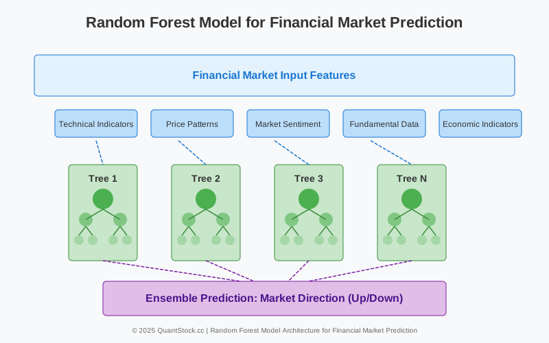
Random forests build upon the concept of decision trees by creating an ensemble of trees trained on different subsets of the data. Each tree independently makes predictions, and the final output is determined by majority vote (for classification) or averaging (for regression). This approach significantly reduces overfitting—a common challenge when applying machine learning to financial markets.
Key Advantages for Financial Applications
Random forests offer several advantages that make them particularly suitable for financial market prediction:
- Robustness to noise and outliers, which are common in financial data
- Built-in feature importance measures that help identify relevant market signals
- Ability to capture non-linear relationships between features
- Reduced risk of overfitting compared to individual decision trees
- Capability to handle mixed data types often present in financial datasets
Feature Engineering for Financial Datasets
The effectiveness of any machine learning model, including random forests, heavily depends on the quality of input features. In financial market prediction, thoughtful feature engineering can significantly enhance model performance.
Technical Indicators as Features
Technical indicators provide valuable information about market trends, momentum, and volatility. Common indicators used as features include:
- Moving averages and their crossovers
- Relative Strength Index (RSI) and other oscillators
- Bollinger Bands and volatility measures
- MACD (Moving Average Convergence Divergence)
- Volume-based indicators
Financial Ratios and Fundamental Data
For longer-term predictions, incorporating fundamental data can improve model performance:
- Price-to-earnings (P/E) ratios
- Earnings growth metrics
- Debt-to-equity ratios
- Cash flow measures
- Market capitalization and liquidity metrics
Market Sentiment Features
Sentiment analysis can provide additional predictive power by capturing market psychology:
- News sentiment scores
- Social media sentiment analysis
- Options market sentiment indicators (put-call ratio)
- Analyst consensus metrics
Implementing Random Forest Models: A Step-by-Step Guide
Let's walk through the process of implementing a random forest model for financial market prediction with Python:
Data Preparation and Preprocessing
The first step involves collecting and preprocessing financial time series data:
      import pandas as pd
      import numpy as np
      from sklearn.ensemble import RandomForestClassifier
      from sklearn.model_selection import train_test_split

      # Load historical market data
      market_data = pd.read_csv('spy_historical_data.csv')

      # Calculate technical indicators
      market_data['SMA_20'] = market_data['Close'].rolling(window=20).mean()
      market_data['SMA_50'] = market_data['Close'].rolling(window=50).mean()
      market_data['RSI'] = calculate_rsi(market_data['Close'], window=14)

      # Calculate returns
      market_data['Daily_Return'] = market_data['Close'].pct_change()

      # Create target variable (e.g., direction of next day's return)
      market_data['Target'] = np.where(market_data['Daily_Return'].shift(-1) > 0, 1, 0)

      # Drop NaN values resulting from rolling windows
      market_data = market_data.dropna()
Feature Selection and Engineering
Selecting and engineering the right features is crucial for model performance:
      # Create additional features
      market_data['SMA_Ratio'] = market_data['SMA_20'] / market_data['SMA_50']
      market_data['Price_to_SMA'] = market_data['Close'] / market_data['SMA_20']
      market_data['Volatility'] = market_data['Daily_Return'].rolling(window=20).std()

      # Add lagged features to capture temporal patterns
      for i in range(1, 6):
          market_data[f'Return_Lag_{i}'] = market_data['Daily_Return'].shift(i)

      # Define features and target
      features = ['SMA_Ratio', 'Price_to_SMA', 'RSI', 'Volatility'] +                 [f'Return_Lag_{i}' for i in range(1, 6)]

      X = market_data[features]
      y = market_data['Target']
Model Training and Validation
Proper validation is essential to ensure the model generalizes well to new market conditions:
      # Split data chronologically (time series data should not be randomly split)
      train_size = int(len(X) * 0.7)
      X_train, X_test = X[:train_size], X[train_size:]
      y_train, y_test = y[:train_size], y[train_size:]

      # Initialize and train the random forest classifier
      rf_model = RandomForestClassifier(
          n_estimators=100,
          max_depth=5,
          min_samples_split=10,
          min_samples_leaf=4,
          random_state=42
      )

      rf_model.fit(X_train, y_train)

      # Evaluate model performance
      from sklearn.metrics import accuracy_score, precision_score, recall_score, f1_score

      y_pred = rf_model.predict(X_test)

      print(f"Accuracy: {accuracy_score(y_test, y_pred):.4f}")
      print(f"Precision: {precision_score(y_test, y_pred):.4f}")
      print(f"Recall: {recall_score(y_test, y_pred):.4f}")
      print(f"F1 Score: {f1_score(y_test, y_pred):.4f}")
Hyperparameter Tuning and Optimization
Fine-tuning the model parameters can significantly improve performance:
      from sklearn.model_selection import GridSearchCV

      # Define parameter grid
      param_grid = {
          'n_estimators': [50, 100, 200],
          'max_depth': [3, 5, 7, 10],
          'min_samples_split': [5, 10, 15],
          'min_samples_leaf': [2, 4, 6, 8]
      }

      # Use TimeSeriesSplit for time series data
      from sklearn.model_selection import TimeSeriesSplit
      tscv = TimeSeriesSplit(n_splits=5)

      # Initialize grid search
      grid_search = GridSearchCV(
          estimator=RandomForestClassifier(random_state=42),
          param_grid=param_grid,
          cv=tscv,
          scoring='f1',
          n_jobs=-1
      )

      # Fit grid search
      grid_search.fit(X_train, y_train)

      # Get best parameters
      best_params = grid_search.best_params_
      print(f"Best parameters: {best_params}")

      # Train model with best parameters
      optimized_rf = RandomForestClassifier(
          **best_params,
          random_state=42
      )
      optimized_rf.fit(X_train, y_train)
Evaluating Model Performance in Financial Context
When evaluating random forest models for financial applications, traditional accuracy metrics may not be sufficient. It's crucial to consider financial performance metrics that reflect real-world trading outcomes.
Beyond Classification Metrics
While accuracy, precision, and recall provide insights into classification performance, financial applications require additional evaluation:
      # Calculate returns based on model predictions
      market_data_test = market_data.iloc[train_size:].copy()
      market_data_test['Predicted'] = y_pred

      # Simulate trading strategy based on predictions
      market_data_test['Strategy_Return'] = np.where(
          market_data_test['Predicted'] == 1,
          market_data_test['Daily_Return'],
          0
      )

      # Calculate cumulative returns
      market_data_test['Cumulative_Market_Return'] = (1 + market_data_test['Daily_Return']).cumprod() - 1
      market_data_test['Cumulative_Strategy_Return'] = (1 + market_data_test['Strategy_Return']).cumprod() - 1

      # Calculate performance metrics
      strategy_return = market_data_test['Cumulative_Strategy_Return'].iloc[-1]
      market_return = market_data_test['Cumulative_Market_Return'].iloc[-1]

      # Calculate Sharpe ratio (assuming risk-free rate of 0 for simplicity)
      strategy_sharpe = market_data_test['Strategy_Return'].mean() / market_data_test['Strategy_Return'].std() * np.sqrt(252)

      print(f"Strategy Return: {strategy_return:.4f}")
      print(f"Market Return: {market_return:.4f}")
      print(f"Strategy Sharpe Ratio: {strategy_sharpe:.4f}")
Analyzing Feature Importance
One advantage of random forests is the ability to determine which features contribute most to prediction accuracy:
      # Get feature importance
      feature_importance = pd.DataFrame({
          'Feature': features,
          'Importance': optimized_rf.feature_importances_
      }).sort_values('Importance', ascending=False)

      print(feature_importance)
Practical Applications and Integration with Trading Systems
To move from model development to practical implementation, we need to integrate the random forest model with a trading system.
Building a Trading Signal Generator
Convert model predictions into actionable trading signals:
      def generate_trading_signals(model, market_data, features):
          """Generate trading signals based on random forest predictions"""
          # Prepare features
          X = market_data[features].copy()

          # Make predictions
          predictions = model.predict(X)
          probabilities = model.predict_proba(X)[:, 1]  # Probability of positive class

          # Create signal based on prediction and confidence
          signals = pd.DataFrame({
              'Date': market_data.index,
              'Prediction': predictions,
              'Confidence': probabilities,
              'Signal': np.where(probabilities > 0.65, 1, np.where(probabilities < 0.35, -1, 0))
          })

          return signals
Implementing a Backtesting Framework
Test the strategy's performance over historical data:
      def backtest_strategy(signals, market_data, initial_capital=10000):
          """Backtest a trading strategy based on signals"""
          # Initialize portfolio
          portfolio = pd.DataFrame({
              'Date': market_data.index,
              'Holdings': 0,
              'Cash': initial_capital,
              'Position_Value': 0,
              'Portfolio_Value': initial_capital
          }).set_index('Date')

          # Iterate through each trading day
          for i in range(1, len(signals)):
              current_date = signals.index[i]
              previous_date = signals.index[i-1]

              # Get current price
              current_price = market_data.loc[current_date, 'Close']

              # Get previous position and cash
              previous_holdings = portfolio.loc[previous_date, 'Holdings']
              previous_cash = portfolio.loc[previous_date, 'Cash']

              # Determine action based on signal
              current_signal = signals.loc[current_date, 'Signal']

              # Execute trades
              if current_signal == 1 and previous_holdings == 0:  # Buy signal
                  shares_to_buy = previous_cash // current_price
                  cash_spent = shares_to_buy * current_price
                  new_holdings = shares_to_buy
                  new_cash = previous_cash - cash_spent
              elif current_signal == -1 and previous_holdings > 0:  # Sell signal
                  cash_received = previous_holdings * current_price
                  new_holdings = 0
                  new_cash = previous_cash + cash_received
              else:  # Hold
                  new_holdings = previous_holdings
                  new_cash = previous_cash

              # Update portfolio
              portfolio.loc[current_date, 'Holdings'] = new_holdings
              portfolio.loc[current_date, 'Cash'] = new_cash
              portfolio.loc[current_date, 'Position_Value'] = new_holdings * current_price
              portfolio.loc[current_date, 'Portfolio_Value'] = new_cash + new_holdings * current_price

          # Calculate returns
          portfolio['Daily_Return'] = portfolio['Portfolio_Value'].pct_change()
          portfolio['Cumulative_Return'] = (1 + portfolio['Daily_Return']).cumprod() - 1

          return portfolio
Implementing Walk-Forward Analysis
To better account for market regime changes, implement a walk-forward testing approach:
      def walk_forward_analysis(market_data, features, target, window_size=252, step_size=63):
          """Implement walk-forward analysis for model validation"""
          results = []

          # Define windows for walk-forward analysis
          for start_idx in range(0, len(market_data) - window_size * 2, step_size):
              end_train_idx = start_idx + window_size
              end_test_idx = end_train_idx + window_size

              # Ensure we have enough data
              if end_test_idx > len(market_data):
                  break

              # Split data
              train_data = market_data.iloc[start_idx:end_train_idx]
              test_data = market_data.iloc[end_train_idx:end_test_idx]

              # Train model
              X_train = train_data[features]
              y_train = train_data[target]

              model = RandomForestClassifier(
                  n_estimators=100,
                  max_depth=5,
                  min_samples_split=10,
                  random_state=42
              )
              model.fit(X_train, y_train)

              # Generate predictions and backtest
              X_test = test_data[features]
              predictions = model.predict(X_test)

              # Calculate performance metrics
              test_data['Predicted'] = predictions
              test_data['Strategy_Return'] = np.where(
                  test_data['Predicted'] == 1,
                  test_data['Daily_Return'],
                  0
              )

              strategy_return = (1 + test_data['Strategy_Return']).prod() - 1
              market_return = (1 + test_data['Daily_Return']).prod() - 1

              results.append({
                  'Period_Start': train_data.index[0],
                  'Period_End': test_data.index[-1],
                  'Strategy_Return': strategy_return,
                  'Market_Return': market_return,
                  'Outperformance': strategy_return - market_return
              })

          return pd.DataFrame(results)
Enhancing Random Forest Models with Advanced Techniques
Several advanced techniques can further improve random forest performance for financial prediction.
Ensemble Stacking
Combine random forests with other algorithms for improved predictions:
      from sklearn.linear_model import LogisticRegression
      from sklearn.svm import SVC
      from sklearn.ensemble import StackingClassifier

      # Define base models
      base_models = [
          ('rf', RandomForestClassifier(n_estimators=100, random_state=42)),
          ('svm', SVC(probability=True, random_state=42))
      ]

      # Define meta-learner
      meta_learner = LogisticRegression()

      # Create stacked model
      stacked_model = StackingClassifier(
          estimators=base_models,
          final_estimator=meta_learner,
          cv=TimeSeriesSplit(n_splits=5)
      )

      # Train stacked model
      stacked_model.fit(X_train, y_train)
Feature Expansion with Market Regimes
Incorporating market regime detection can enhance model adaptability:
      # Identify market regimes using volatility
      def identify_market_regimes(returns, window=20):
          volatility = returns.rolling(window=window).std() * np.sqrt(252)

          # Define regimes based on volatility levels
          regimes = pd.Series(index=volatility.index, data=1)  # Default: normal regime
          regimes[volatility > volatility.quantile(0.8)] = 2    # High volatility
          regimes[volatility < volatility.quantile(0.2)] = 0    # Low volatility

          return regimes

      # Add market regime feature
      market_data['Regime'] = identify_market_regimes(market_data['Daily_Return'])

      # Add regime-specific features
      for regime in [0, 1, 2]:
          for feature in features:
              market_data[f'{feature}_Regime_{regime}'] = np.where(
                  market_data['Regime'] == regime,
                  market_data[feature],
                  0
              )
Integration with QuantStock's Portfolio Optimization Tools
The random forest prediction model can be integrated with QuantStock's portfolio optimization tools to create a more comprehensive investment strategy.
Signal-Based Portfolio Allocation
Use model predictions as inputs for portfolio optimization:
      # Generate predictions for multiple assets
      def generate_multi_asset_signals(models, market_data_dict, features):
          """Generate signals for multiple assets"""
          all_signals = {}

          for asset, model in models.items():
              asset_data = market_data_dict[asset]
              signals = generate_trading_signals(model, asset_data, features)
              all_signals[asset] = signals

          return all_signals

      # Create portfolio weights based on signal confidence
      def optimize_portfolio_weights(signals_dict, optimization_method='equal_weight'):
          """Allocate portfolio based on signals"""
          # Get dates shared by all assets
          common_dates = set.intersection(*[set(signals.index) for signals in signals_dict.values()])
          common_dates = sorted(list(common_dates))

          # Initialize weights dictionary
          weights = {date: {} for date in common_dates}

          # Allocate weights based on selected method
          if optimization_method == 'equal_weight':
              # Equal weight among positive signals
              for date in common_dates:
                  positive_signals = [asset for asset, signals in signals_dict.items()
                                    if signals.loc[date, 'Signal'] == 1]

                  if positive_signals:
                      weight = 1.0 / len(positive_signals)
                      for asset in signals_dict.keys():
                          weights[date][asset] = weight if asset in positive_signals else 0.0
                  else:
                      # No positive signals, stay in cash
                      for asset in signals_dict.keys():
                          weights[date][asset] = 0.0

          elif optimization_method == 'confidence_weighted':
              # Weight proportional to prediction confidence
              for date in common_dates:
                  # Get confidence values for assets with positive signals
                  confidences = {asset: signals.loc[date, 'Confidence']
                               for asset, signals in signals_dict.items()
                               if signals.loc[date, 'Signal'] == 1}

                  if confidences:
                      # Normalize confidences to sum to 1
                      total_confidence = sum(confidences.values())
                      for asset in signals_dict.keys():
                          weights[date][asset] = confidences.get(asset, 0) / total_confidence
                  else:
                      # No positive signals, stay in cash
                      for asset in signals_dict.keys():
                          weights[date][asset] = 0.0

          return weights
Hybrid Approach: Combining Systematic and AI-Driven Strategies
A hybrid approach can leverage the strengths of both systematic portfolio optimization and machine learning predictions:
      def hybrid_portfolio_strategy(market_data, ml_signals, efficient_frontier_weights, alpha=0.5):
          """Combine ML signals with efficient frontier optimization"""
          # Initialize hybrid weights
          hybrid_weights = {}

          for date in ml_signals.index:
              if date in efficient_frontier_weights:
                  # Combine weights using alpha parameter
                  if ml_signals.loc[date, 'Signal'] == 1:
                      # Use alpha to weight between ML signal (overweight) and efficient frontier
                      hybrid_weights[date] = {
                          'ML_Weight': alpha,
                          'EF_Weight': 1 - alpha
                      }
                  elif ml_signals.loc[date, 'Signal'] == -1:
                      # ML suggests reducing exposure
                      hybrid_weights[date] = {
                          'ML_Weight': 0,
                          'EF_Weight': 0.5  # Reduce efficient frontier allocation
                      }
                  else:
                      # Neutral signal, rely more on efficient frontier
                      hybrid_weights[date] = {
                          'ML_Weight': 0,
                          'EF_Weight': 1.0
                      }

          return hybrid_weights
Conclusion: Deploying Your Random Forest Models in Production
Successfully implementing random forest models for financial market prediction requires careful attention to data preparation, feature engineering, model validation, and integration with existing trading systems.
As with any machine learning approach in finance, it's crucial to continuously monitor model performance and be prepared to adapt to changing market conditions. Random forests provide a powerful framework for financial prediction, but they require ongoing maintenance and regular retraining to maintain their effectiveness.
By combining random forest predictions with traditional portfolio optimization techniques, as offered by QuantStock's portfolio optimization platform, investors can develop more robust and adaptive investment strategies. The integration of machine learning signals with efficient frontier analysis represents a powerful approach to modern portfolio management—blending the data-driven insights of quantitative methods with the adaptive learning capabilities of artificial intelligence.
For further exploration of related topics, consider reading our articles on machine learning for asset price prediction and factor investing and systematic exposures.
Free Trading Math & Risk Cheat Sheet
Every key formula in one PDF: breakeven win rates, expectancy, position sizing, drawdown recovery, volatility drag, VaR and CVaR. Plus occasional emails when we publish new quant tools.